Available Optimizers: How to Find Maximum A Posteriori?

library(gips)

?find_MAP()

What are we optimizing?

The goal of the find_MAP() is to find the permutation $\sigma$ that maximizes the a posteriori probability (MAP - Maximum A Posteriori). Such a permutation represents the most plausible symmetry given the data.

This a posteriori probability function is described in-depth in the Bayesian model selection section of the vignette("Theory", package="gips"), also available as a pkgdown page. gips can calculate the logarithm of it by the log_posteriori_of_gips() function. In the following paragraphs, we will refer to this a posteriori probability function as $f(\sigma)$. We have $f(\sigma) > 0$.

Available optimizers

The space of permutations is enormous - for the permutation of size $p$, the space of all permutations is of size $p!$ ($p$ factorial). Even for $p=12$, this space is practically impossible to browse. This is why find_MAP() implements multiple (3) optimizers to choose from:

• "brute_force", "BF", "full" | recommend for $p\le 9$.
• "Metropolis_Hastings", "MH" | recommend for $p\ge 10$.
• "hill_climbing", "HC"

Note on computation time

The max_iter parameter functions differently in Metropolis-Hastings and hill climbing.

For Metropolis-Hastings, it computes a posteriori of max_iter permutations, whereas for hill climbing, it computes ${p\choose 2} \cdot$max_iter of them.

In the case of the Brute Force optimizer, it computes all $f(\sigma)$ values. The number of all different $\sigma$s follows OEIS sequence A051625.

Brute Force

It searches through the whole space at once.

This is the only optimizer that will certainly find the actual MAP Estimator.

Brute Force is only recommended for small spaces ($p \le 9$). It can also browse bigger spaces, but the required time is probably too long. We tested how much time it takes to browse with Brute Force (Apple M2, single core), and we show the time in the table below:

p=2	p=3	p=4	p=5	p=6	p=7	p=8	p=9	p=10
0.005 sec 1	0.010 sec	0.025 sec	0.075 sec	0.3 sec	1.8 sec	13 sec	1.8 min	47 min

Example

perm_size <- 6
mu <- runif(perm_size, -10, 10) # Assume we don't know the mean
sigma_matrix <- matrix(
  data = c(
    1.0, 0.8, 0.6, 0.4, 0.6, 0.8,
    0.8, 1.0, 0.8, 0.6, 0.4, 0.6,
    0.6, 0.8, 1.0, 0.8, 0.6, 0.4,
    0.4, 0.6, 0.8, 1.0, 0.8, 0.6,
    0.6, 0.4, 0.6, 0.8, 1.0, 0.8,
    0.8, 0.6, 0.4, 0.6, 0.8, 1.0
  ),
  nrow = perm_size, byrow = TRUE
) # the real covariance matrix, that we want to estimate, is invariant under permutation (1,2,3,4,5,6)
number_of_observations <- 13
Z <- withr::with_seed(2022,
  code = MASS::mvrnorm(number_of_observations, mu = mu, Sigma = sigma_matrix)
)

Show/hide data preparation

Let’s say we have the data Z from the unknown process:

dim(Z)
#> [1] 13  6
number_of_observations <- nrow(Z) # 13
perm_size <- ncol(Z) # 6
S <- cov(Z) # Assume we have to estimate the mean

g <- gips(S, number_of_observations)

g_map <- find_MAP(g, optimizer = "brute_force")
#> ================================================================================
g_map
#> The permutation (1,2,3,4,5,6):
#>  - was found after 362 posteriori calculations;
#>  - is 28979.967 times more likely than the () permutation.

Brute Force needed 362 calculations, as predicted in OEIS sequence A051625 for $p = 6$.

Metropolis-Hastings

This optimizer implements the Second approach from [1, Sec 4.1.2].

It uses the Metropolis-Hastings algorithm to optimize the space; see Wikipedia. This algorithm used in this context is a special case of the Simulated Annealing the reader may be more familiar with; see Wikipedia.

Short description

In every iteration $i$, an algorithm considers a permutation, say, $\sigma_i$. Then a random transposition is drawn uniformly $t_i = (j,k)$, and the value of $f(\sigma_i \circ t_i)$ is computed.

• If a new value is bigger than the previous one (i.e., $f(\sigma_i \circ t_i) \ge f(\sigma_i)$), then we set $\sigma_{i+1} = \sigma_i \circ t_i$.
• If a new value is smaller ($f(\sigma_i \circ t_i) < f(\sigma_i)$), then we will choose $\sigma_{i+1} = \sigma_i \circ t_i$ with probability $\frac{f(\sigma_i \circ t_i)}{f(\sigma_i)}$. Otherwise, we set $\sigma_{i+1} = \sigma_i$ with complementary probability $1 - \frac{f(\sigma_i \circ t_i)}{f(\sigma_i)}$.

The final value is the best $\sigma$ ever computed.

Notes

This algorithm was tested in multiple settings and turned out to be an outstanding optimizer for this problem. Especially given it does not need any hyperparameters tuned.

The only parameter it depends on is max_iter, which determines the number of steps described above. One should choose this number rationally. When decided too small, there is a missed opportunity to find a much better permutation. When decided too big, there is a lost time and computational power that does not lead to growth. We recommend plotting the convergence plot with a logarithmic OX scale: plot(g_map, type = "best", logarithmic_x = TRUE), then decide if the line has flattened already. Keep in mind that the OY scale is also logarithmic. For example, a marginal change on the OY scale could mean $10000$times the change in A Posteriori.

For more information about continuing the optimization, see the Continuing the optimization section below.

This algorithm has been analyzed extensively by statisticians. Thanks to the ergodic theorem, the frequency of visits to a given state converges almost surely to the probability of that state. This is the approach explained in [1, Sec.4.1.2] and shown in [1, Sec. 5.2]. One can obtain estimates of posterior probabilities by setting return_probabilities = TRUE.

Example

perm_size <- 70
mu <- runif(perm_size, -10, 10) # Assume we don't know the mean
sigma_matrix <- (function(A) {
  t(A) %*% A
})(matrix(rnorm(perm_size * perm_size), nrow = perm_size))
# sigma_matrix is the real covariance matrix, that we want to estimate
number_of_observations <- 50
Z <- withr::with_seed(2022,
  code = MASS::mvrnorm(number_of_observations, mu = mu, Sigma = sigma_matrix)
)

Show/hide data preparation

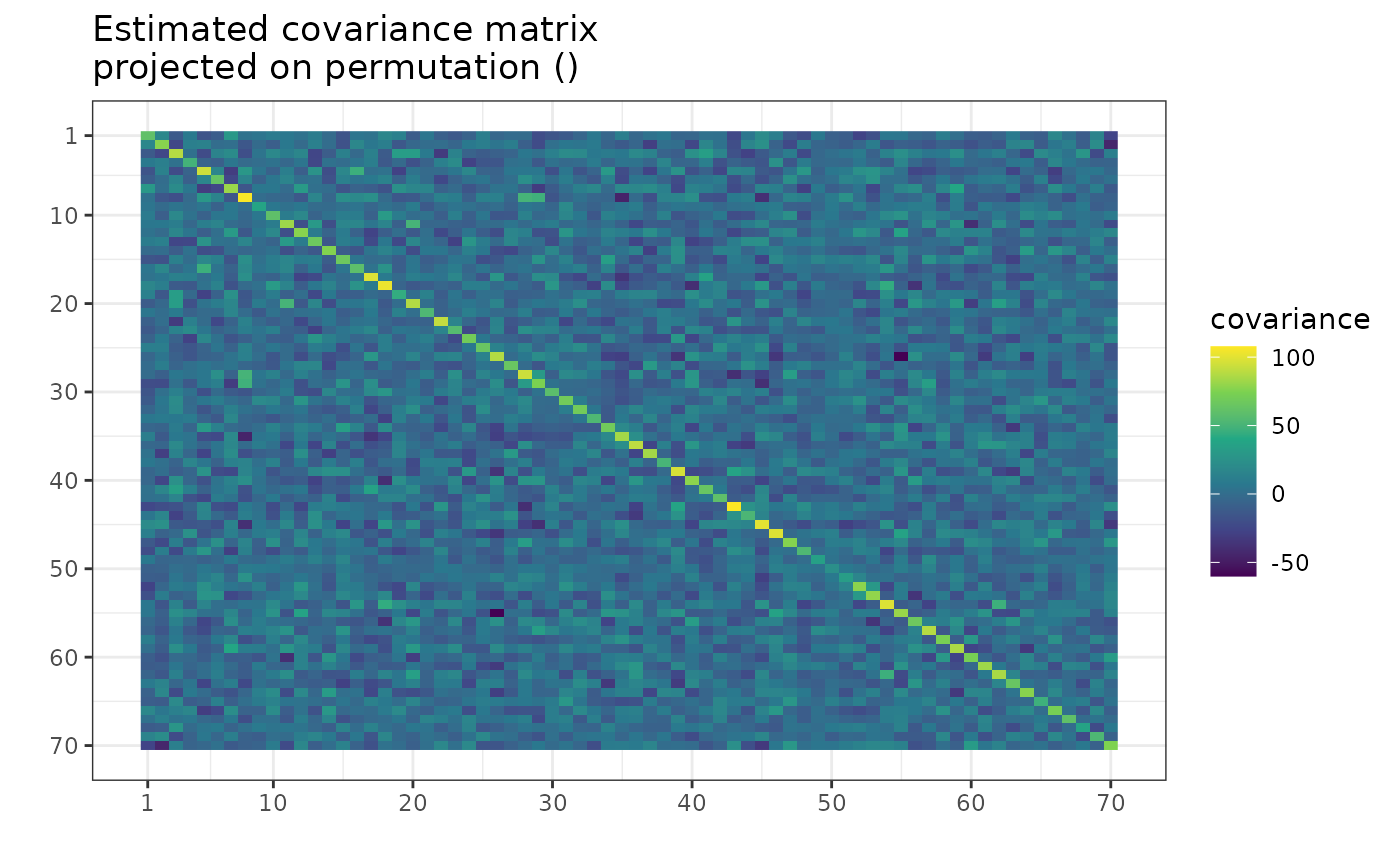
Let’s say we have the data Z from the unknown process:

dim(Z)
#> [1] 50 70
number_of_observations <- nrow(Z) # 50
perm_size <- ncol(Z) # 70
S <- cov(Z) # Assume we have to estimate the mean

g <- gips(S, number_of_observations)
suppressMessages( # message from ggplot2
  plot(g, type = "heatmap") +
    ggplot2::scale_x_continuous(breaks = c(1, 10, 20, 30, 40, 50, 60, 70)) +
    ggplot2::scale_y_reverse(breaks = c(1, 10, 20, 30, 40, 50, 60, 70))
)

g_map <- find_MAP(g, max_iter = 150, optimizer = "Metropolis_Hastings")
#> ===============================================================================
g_map
#> The permutation (1,34,64,27,60,40,26,14,13,53,62,22,11,41,21,7,29,48,24,30,46,57,38,16,23,18,20,10,59,35,32,69,54,17,2,58,31,8,49,66,52,15,47,37,45,50,51,3,63,43,68,33,19,44,55,6,9,4,36,56,25,39,61,70,42,5,67):
#>  - was found after 150 posteriori calculations;
#>  - is 5.34e+648 times more likely than the () permutation.

After just a hundred and fifty iterations, the found permutation is unimaginably more likely than the $_0 = $ () permutation.

plot(g_map, type = "best", logarithmic_x = TRUE)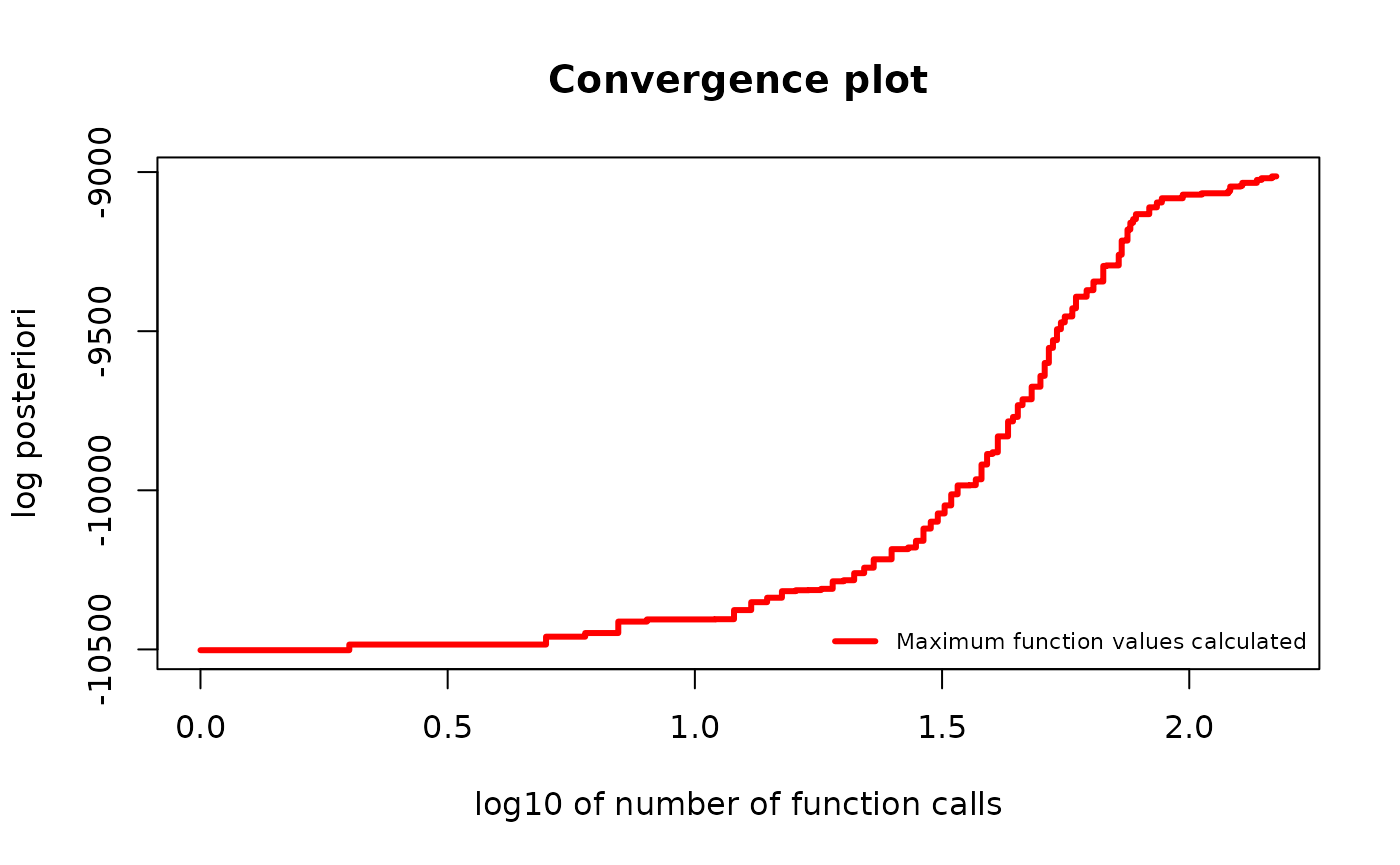

Hill climbing

It uses the Hill climbing algorithm to optimize the space; see Wikipedia.

It is performing the local optimization iteratively.

Short description

In every iteration $i$, an algorithm considers a permutation; call it $\sigma_i$. Then, all the values of $f(\sigma_i \circ t)$ are computed for every possible transposition $t = (j,k)$. Then the next $\sigma_{i+1}$ will be the one with the biggest value:

$$\sigma_{i+1} = argmax_{\text{perm} \in \text{neighbors}(\sigma_{i})}\{f(perm)\}$$

Where: $$\text{neighbors}(\sigma) = \{\sigma \circ (j,k) : 1 \le j < k \le \text{p}\}$$

The algorithm ends when all neighbors are less likely, or the max_iter is achieved. In the first case, the algorithm will finish at a local maximum, but there is no guarantee that this is also the global maximum.

Pseudocode

hill_climb <- function(g, max_iter) {
  perm <- g[[1]]
  perm_log_f <- log_posteriori_of_gips(g)
  perm_size <- attr(perm, "size")
  S <- attr(g, "S")
  number_of_observations <- attr(g, "number_of_observations")

  best_neighbor <- NULL
  best_neighbor_log_f <- -Inf

  i <- 1

  while (perm_i_minus_1_log_f < perm_i_log_f && i < max_iter) {
    best_neighbor <- NULL
    best_neighbor_log_f <- -Inf

    for (j in 1:(perm_size - 1)) {
      for (k in (j + 1):perm_size) {
        t <- c(j, k)
        neighbor <- gips:::compose_with_transposition(perm, t)
        neighbor_log_f <- log_posteriori_of_gips(gips(
          S, number_of_observations,
          perm = neighbor
        ))

        if (neighbor_log_f > best_neighbor_log_f) {
          best_neighbor <- neighbor
          best_neighbor_log_f <- neighbor_log_f
        } # end if
      } # end for k
    } # end for j
    i <- i + 1

    perm_i_minus_1_log_f <- perm_i_log_f

    perm_i <- best_neighbor
    perm_i_log_f <- best_neighbor_log_f
  } # end while

  return(perm_i)
}

Show/hide pseudocode

Example

perm_size <- 25
mu <- runif(perm_size, -10, 10) # Assume we don't know the mean
sigma_matrix <- (function(A) {
  t(A) %*% A
})(matrix(rnorm(perm_size * perm_size), nrow = perm_size))
# sigma_matrix is the real covariance matrix, that we want to estimate
number_of_observations <- 20
Z <- withr::with_seed(2022,
  code = MASS::mvrnorm(number_of_observations, mu = mu, Sigma = sigma_matrix)
)

Show/hide data preparation

Let’s say we have the data Z from the unknown process:

dim(Z)
#> [1] 20 25
number_of_observations <- nrow(Z) # 20
perm_size <- ncol(Z) # 25
S <- cov(Z) # Assume we have to estimate the mean

g <- gips(S, number_of_observations)
plot(g, type = "heatmap")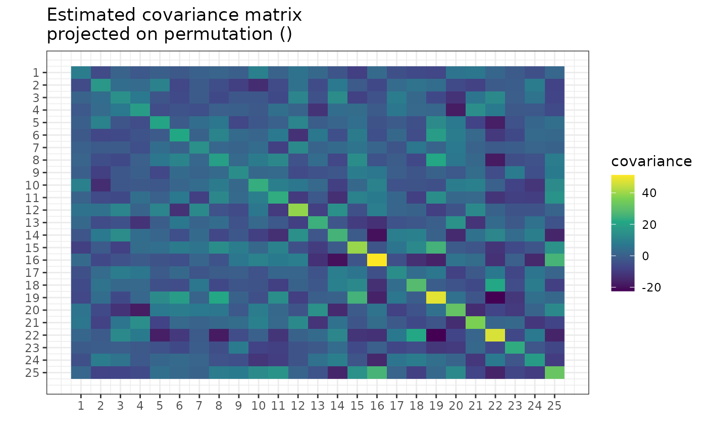

g_map <- find_MAP(g, max_iter = 2, optimizer = "hill_climbing")
#> ================================================================================
#> Warning: Hill Climbing algorithm did not converge in 2 iterations!
#> ℹ We recommend to run the `find_MAP(optimizer = 'continue')` on the acquired output.
#> Warning: The found permutation has n0 = 24, which is bigger than the number_of_observations = 20.
#> ℹ The covariance matrix invariant under the found permutation does not have the likelihood properly defined.
#> ℹ For a more in-depth explanation, see the 'Project Matrix - Equation (6)' section in the `vignette('Theory', package = 'gips')` or its pkgdown page: https://przechoj.github.io/gips/articles/Theory.html.
g_map
#> The permutation (11,15)(13,24):
#>  - was found after 601 posteriori calculations;
#>  - is 2.132e+8 times more likely than the () permutation.
plot(g_map, type = "best")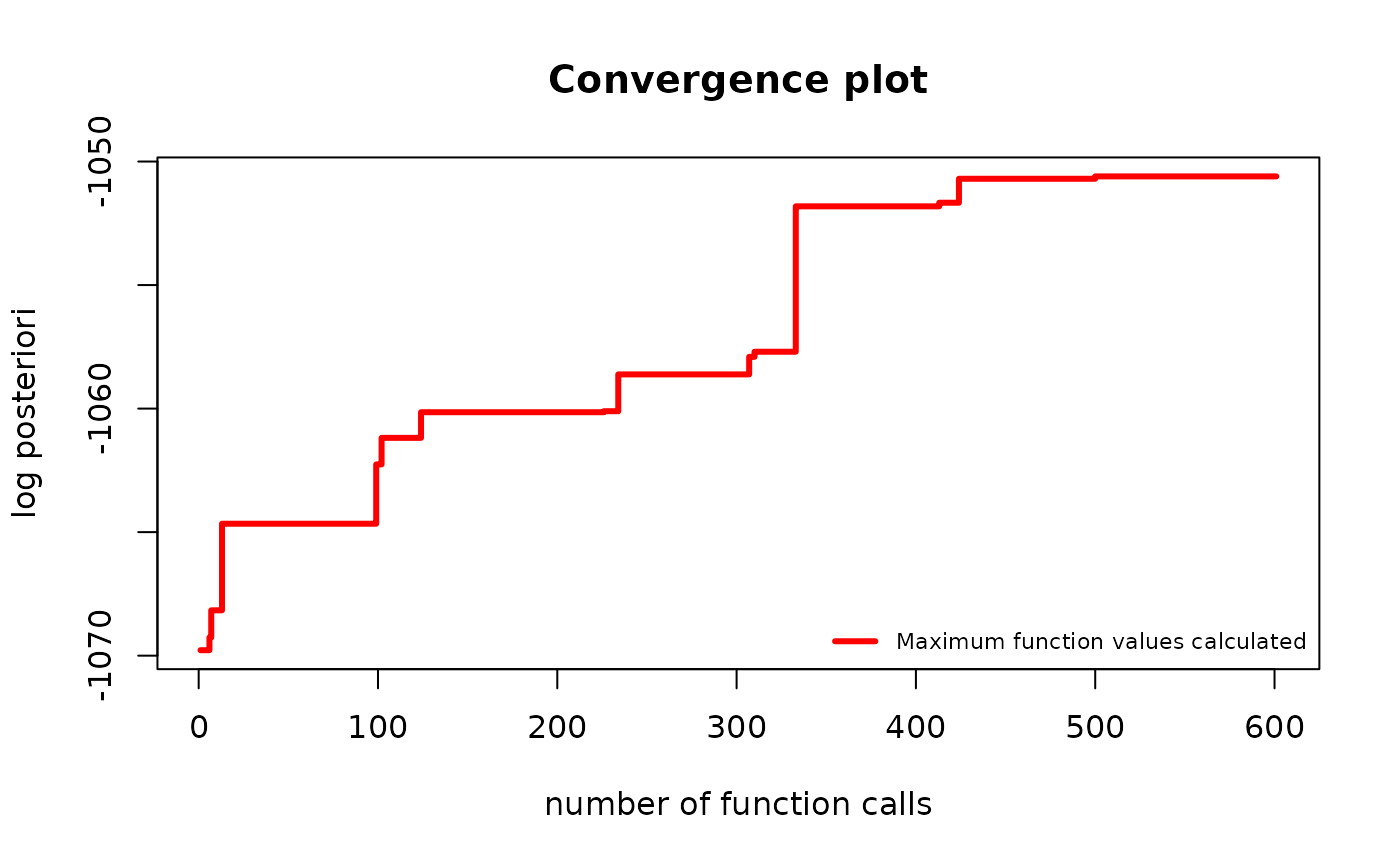

The above warnings are expected.

Continuing the optimization

When max_iter is reached during Metropolis-Hastings or hill climbing, the optimization stops and returns the result. Users are encouraged to plot the result and determine if it has converged. If necessary, users can continue the optimization, as shown below.

# the same code as for generating example for Metripolis-Hastings above

perm_size <- 70
mu <- runif(perm_size, -10, 10) # Assume we don't know the mean
sigma_matrix <- (function(A) {
  t(A) %*% A
})(matrix(rnorm(perm_size * perm_size), nrow = perm_size))
# sigma_matrix is the real covariance matrix, that we want to estimate
number_of_observations <- 50
Z <- withr::with_seed(2022,
  code = MASS::mvrnorm(number_of_observations, mu = mu, Sigma = sigma_matrix)
)

dim(Z)
#> [1] 50 70
number_of_observations <- nrow(Z) # 50
perm_size <- ncol(Z) # 70
S <- cov(Z) # Assume we have to estimate the mean

Show/hide data preparation

g <- gips(S, number_of_observations)

g_map <- find_MAP(g, max_iter = 50, optimizer = "Metropolis_Hastings")
#> ==============================================================================
plot(g_map, type = "best")

The algorithm was still significantly improving the permutation. It is reasonable to continue it:

g_map2 <- find_MAP(g_map, max_iter = 100, optimizer = "continue")
#> ===============================================================================
plot(g_map2, type = "best")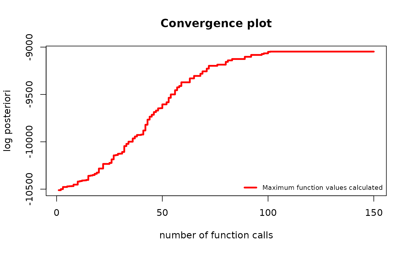

The improvement has slowed down significantly. It is fair to stop the algorithm here. Keep in mind the y scale is logarithmic. The visually “small” improvement between 100 and 150 iterations was huge, $10^{52}$ times the posteriori.

Additional parameters

The find_MAP() function has two additional parameters: show_progress_bar and save_all_perms, which can be set to TRUE or FALSE.

When show_progress_bar = TRUE, gips will print “=” characters on the console during optimization. Remember that when the user sets the return_probabilities = TRUE, a second progress bar will indicate the calculation of the probabilities after optimization.

The save_all_perms = TRUE will save all visited permutations in the outputted object, which significantly increases the required RAM. For instance, with $p=150$ and max_perm = 150000, we needed 400 MB to store it, whereas save_all_perms = FALSE only required 2 MB. However, save_all_perms = TRUE is necessary for return_probabilities = TRUE or more complex path analysis.

Discussion

We are also considering implementing the First approach from [1] in the future. The Markov chain travels along cyclic groups rather than permutations in this approach.

We encourage everyone to discuss on available and potential new optimizers on ISSUE#21. One can also see why some optimizers were implemented but not yet added to gips there.

References

[1] Piotr Graczyk, Hideyuki Ishi, Bartosz Kołodziejek, Hélène Massam. “Model selection in the space of Gaussian models invariant by symmetry.” The Annals of Statistics, 50(3) 1747-1774 June 2022. arXiv link; DOI: 10.1214/22-AOS2174

[2] “Learning permutation symmetries with gips in R” by gips developers Adam Chojecki, Paweł Morgen, and Bartosz Kołodziejek, Journal of Statistical Software.