A Gentle Introduction to Modeling with gips

The problem

Quite often, we have too little data to perform valid inferences. Consider the situation with multivariate Gaussian distribution, where we have few observations compared to the number of variables. For example, that’s the case for graphical models used in biology or medicine. In such a setting, the usual way of finding the covariance matrix (the maximum likelihood method) isn’t statistically applicable. What now?

Invariance by permutation

Sometimes, the interchange of variables in the vector does not change its distribution. In the multivariate Gaussian case, it would mean that they have the same variances and covariances with other respective variables. For instance, in the following covariance matrix, variables X1 and X3 are interchangeable, meaning that vectors (X1, X2, X3) and (X3, X2, X1) have the same distribution.

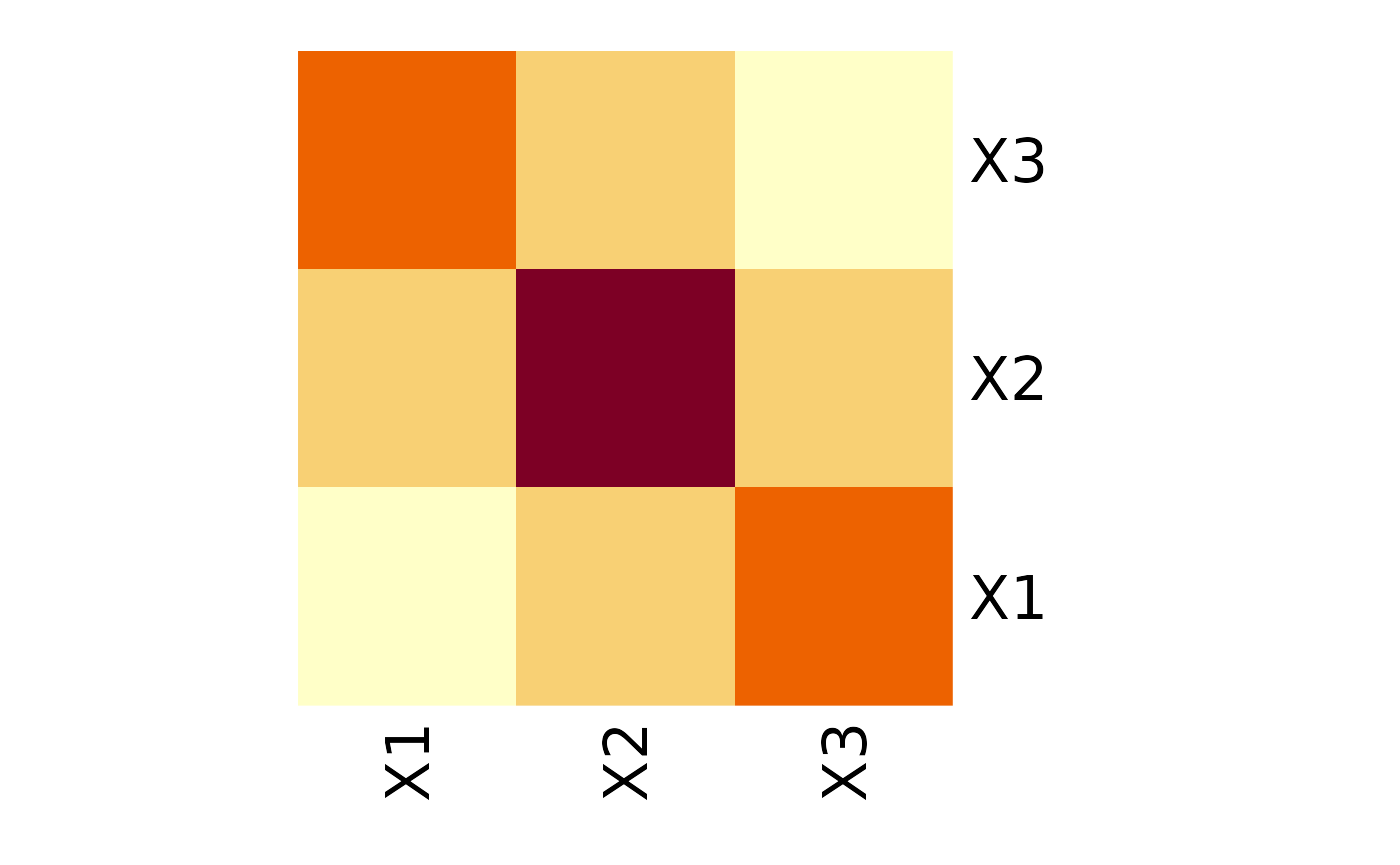
Now, we can state this interchangeability property in terms of permutations. In our case, the distribution of (X1, X2, X3) is invariant by permutation ( $1\mapsto3$ , $3\mapsto1$ ), or in cyclic form $(1,3)(2)$ . This is equivalent to saying that swapping the first with the third row and then swapping the first and third columns of the covariance matrix results in the same matrix. Then we say that this covariance matrix is invariant by permutation.

Of course, in the samples collected in the real world, no perfect equalities will be observed. Still, if the respective values in the (poorly) estimated covariance matrix were close, adopting a particular assumption about invariance by permutation would be a reasonable step.

Package `gips`

We propose creating a set of constraints on the covariance matrix to use the maximum likelihood method. The constraint we consider is - none other than - invariance under permutation symmetry.

This package provides a way to find a reasonable permutation to be used as a constraint in covariance matrix estimation. In this case, reasonable means maximizing the Bayesian posterior distribution when using a Wishart-like distribution on symmetric, positive definite matrices as a prior. The idea, exact formulas, and algorithm sketch are explored in another vignette that can be accessed by vignette("Theory", package="gips") or on its pkgdown page.

For an in-depth analysis of the package performance, capabilities, and comparison with other packages, see the article “Learning permutation symmetries with gips in R” by gips’ developers Adam Chojecki, Paweł Morgen, and Bartosz Kołodziejek, Journal of Statistical Software.

Practical example

Let’s examine 12 books’ thick, height, and breadth data:

library(gips)

Z <- DAAG::oddbooks[, c(1, 2, 3)]

We suspect books from this dataset were printed with $\sqrt{2}$ aspect ratio as in popular A-series paper size. Therefore, we can use this expert knowledge in the analysis and unify the data for height and width:

Z$height <- Z$height / sqrt(2)

Now, let’s plot the data:

number_of_observations <- nrow(Z) # 12
p <- ncol(Z) # 3

S <- cov(Z)
round(S, 1)
#>         thick height breadth
#> thick    72.7  -28.5   -31.7
#> height  -28.5   12.7    14.6
#> breadth -31.7   14.6    17.2
g <- gips(S, number_of_observations)
plot_cosmetic_modifications(plot(g, type = "heatmap")) +
  ggplot2::ggtitle("Standard, MLE estimator\nof a covariance matrix")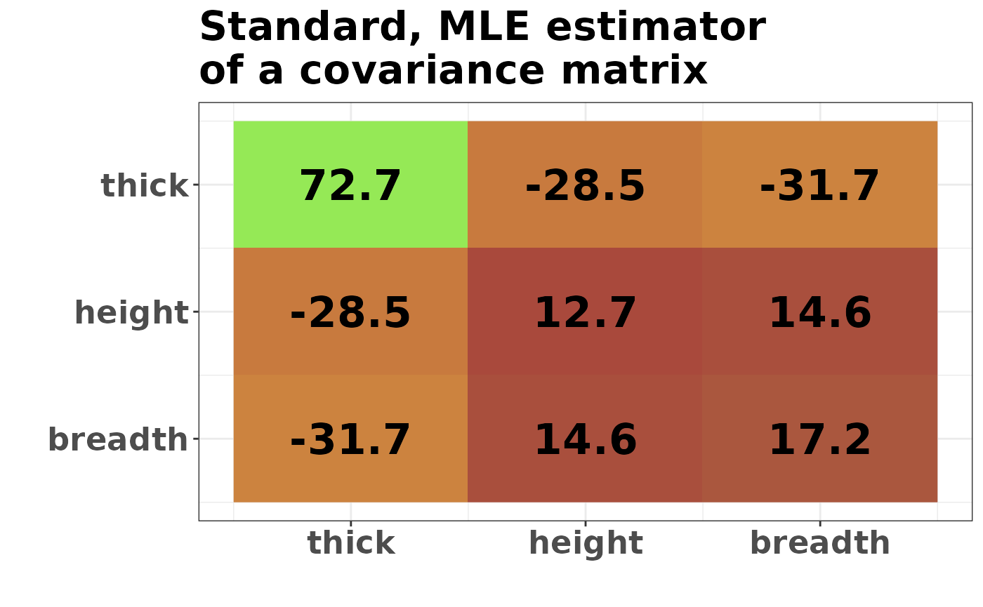

We can see similarities between columns 2 and 3, representing the book’s height and breadth. In particular, the covariance between [1,2] is very similar to [1,3], and the variance of [2] is similar to the variance of [3]. Those are not surprising, given the data interpretation (after the rescaling of height that we did).

Let’s see what the gips will tell about this data:

g_map <- find_MAP(g,
  optimizer = "brute_force",
  return_probabilities = TRUE, save_all_perms = TRUE
)
#> ================================================================================
#> ================================================================================
#> ================================================================================

g_map
#> The permutation (2,3):
#>  - was found after 5 posteriori calculations;
#>  - is 1.305 times more likely than the () permutation.
get_probabilities_from_gips(g_map)
#>          (2,3)             ()          (1,3)        (1,2,3)          (1,2) 
#> 0.566078057717 0.433908667868 0.000006728772 0.000004683290 0.000001862353

find_MAP found the symmetry represented by permutation (2,3).

plot_cosmetic_modifications(plot(g_map, type = "heatmap"))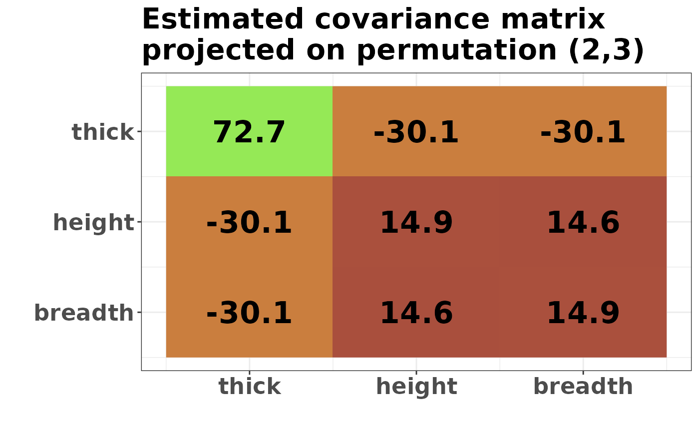

round(project_matrix(S, g_map), 1)
#>         thick height breadth
#> thick    72.7  -30.1   -30.1
#> height  -30.1   14.9    14.6
#> breadth -30.1   14.6    14.9

The result depends on two input parameters, delta and D_matrix. By default, they are set to 3 and diag(p) * d, respectively, where d = mean(diag(S)). The method is not scale-invariant, so we recommend running gips for different values of D_matrix of the form D_matrix = d * diag(p), where d $\in \mathbb{R}^+$ ). The impact analysis of those can be read in [2] in section 3.2. Hyperparameter’s influence.

Theoretic example

library(gips)

toy_example_data
#>            [,1]     [,2]     [,3]      [,4]       [,5]
#> [1,]  -5.554883 7.466693 2.444659 -5.757642  -9.374783
#> [2,] -11.330708 1.700968 2.756588 -5.623130  -8.560550
#> [3,] -10.579451 3.914784 2.327188 -7.085606 -10.115170
#> [4,] -12.634411 4.881232 1.248641 -8.067525 -11.114509

dim(toy_example_data)
#> [1] 4 5
number_of_observations <- nrow(toy_example_data) # 4
p <- ncol(toy_example_data) # 5

S <- cov(toy_example_data)

sum(eigen(S)$values > 0.00000001)
#> [1] 3

Note that the rank of the S matrix is 3, despite the number_of_observations being 4. This is because cov() estimated the mean on every column to compute S.

We want to find reasonable additional assumptions on S to make it easier to estimate.

g <- gips(S, number_of_observations)

plot(g, type = "heatmap")

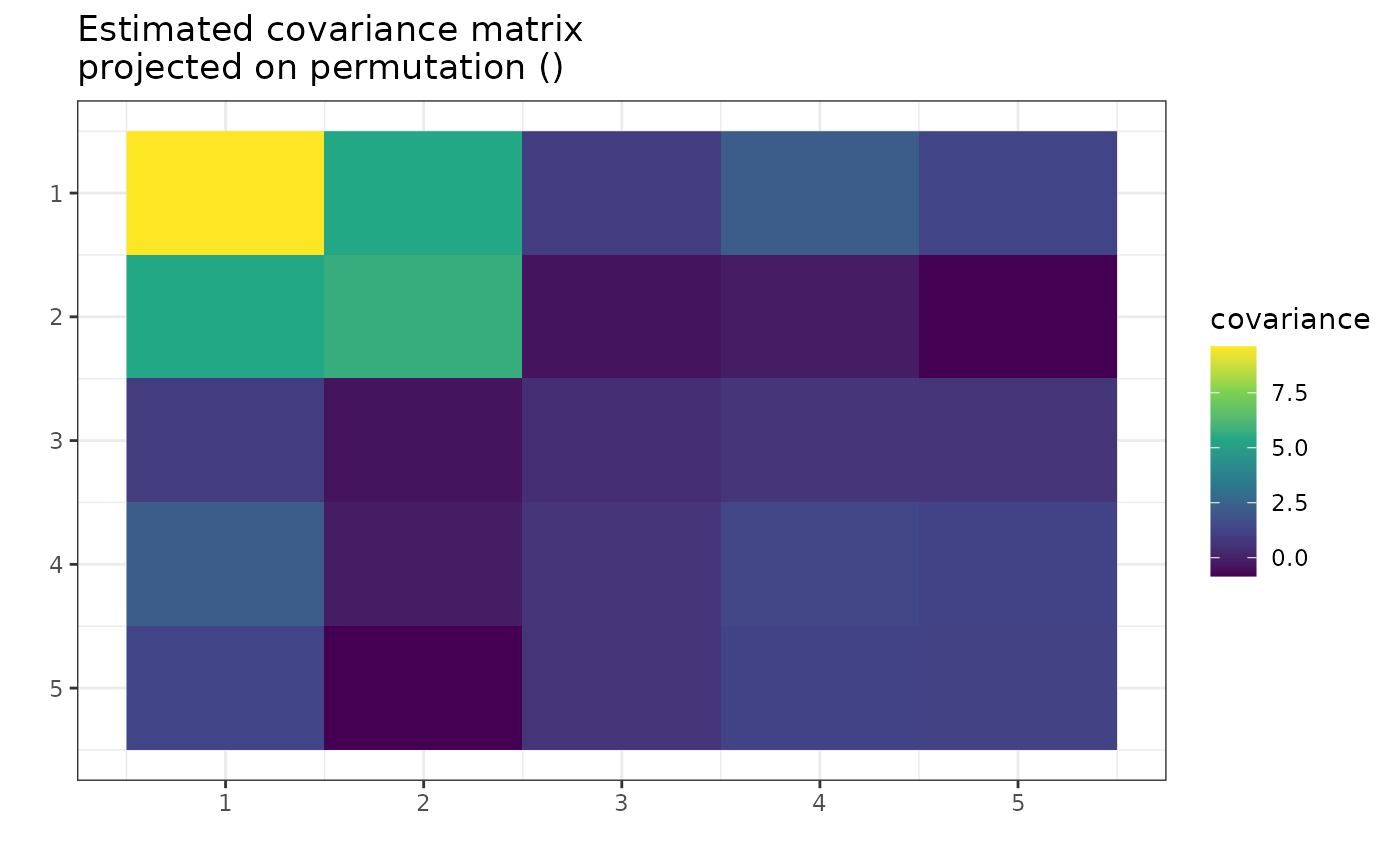
Looking at the plot, one can see the similarities between columns 3, 4, and 5. They have similar variance and covariance to each other. The 3 and 5 have similar covariance with columns 1 and 2. However, the 4 is also close.

Let’s see if gips will find the relationship:

g_map <- find_MAP(g,
  optimizer = "brute_force",
  return_probabilities = TRUE, save_all_perms = TRUE
)
#> ================================================================================
#> ================================================================================
#> ================================================================================

plot(g_map, type = "heatmap")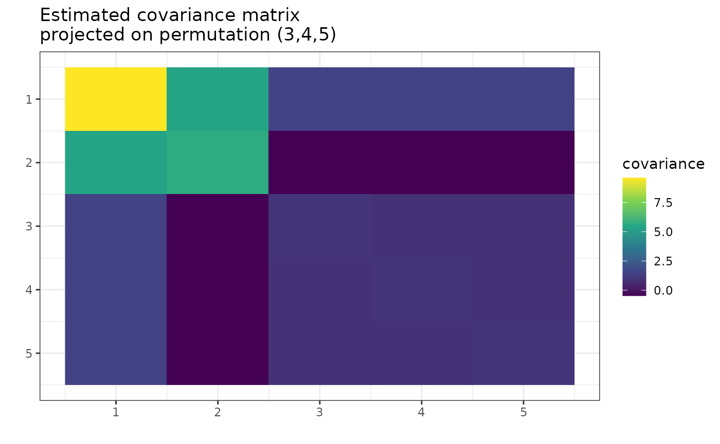

gips decided that $(3,4,5)$ was the most reasonable assumption. Let’s see how much better it is:

g_map
#> The permutation (3,4,5):
#>  - was found after 67 posteriori calculations;
#>  - is 3.63 times more likely than the () permutation.

This assumption is over 3 times more believable than making no assumption. Let’s examine how reasonable are other possible assumptions:

get_probabilities_from_gips(g_map)
#>      (3,4,5)      (2,4,5) (1,2)(3,4,5)    (2,3,5,4)        (4,5)        (3,5) 
#>  0.061991931  0.056959514  0.048479131  0.040410788  0.038027185  0.037829891 
#>        (3,4)    (2,3,4,5)    (2,4,3,5)   (2,4)(3,5)      (2,3,5)   (1,2)(3,5) 
#>  0.035085538  0.034415530  0.033895061  0.031448291  0.029438098  0.026938644 
#>   (1,2)(3,4)   (2,5)(3,4)   (1,2)(4,5)      (2,3,4)        (2,5)        (2,4) 
#>  0.026167559  0.025906388  0.025384163  0.024145834  0.024081717  0.020399181 
#> (1,2,4)(3,5)    (1,4,2,5)   (2,3)(4,5)           ()  (1,2,3,5,4)    (1,2,5,4) 
#>  0.019323499  0.018904417  0.018141398  0.017079855  0.016588093  0.016298998 
#> (1,2,5)(3,4)    (1,2,4,5)        (1,2) (1,4)(2,3,5)        (2,3)  (1,2,3,4,5) 
#>  0.015996810  0.013635218  0.013223117  0.012292494  0.011350938  0.010572077 
#>  (1,2,5,3,4) (1,2,3)(4,5)  (1,2,4,5,3)   (1,4)(2,5) (1,3)(2,4,5)  (1,2,4,3,5) 
#>  0.010280022  0.010147160  0.009968266  0.009810562  0.009448103  0.009398996 
#>    (1,2,3,5)      (1,2,4)      (1,2,5) (1,5)(2,3,4)    (1,3,2,5)    (1,2,3,4) 
#>  0.009168309  0.009011297  0.008941143  0.008833158  0.008315048  0.008279742 
#>  (1,2,5,4,3)    (1,3,2,4)   (1,4)(3,5)   (1,5)(2,4)    (1,2,5,3)      (1,2,3) 
#>  0.008007561  0.006254947  0.005565898  0.005389584  0.004968273  0.004515910 
#>   (1,4)(2,3)   (1,5)(2,3)    (1,2,4,3)   (1,3)(4,5)   (1,5)(3,4) (1,3,4)(2,5) 
#>  0.004287814  0.004249572  0.003919107  0.003875914  0.003868923  0.003383014 
#>        (1,4)   (1,3)(2,5)        (1,5) (1,3,5)(2,4)        (1,3)      (1,4,5) 
#>  0.003272443  0.002762345  0.002701743  0.002404967  0.002143353  0.002045112 
#> (1,4,5)(2,3)      (1,3,4)   (1,3)(2,4)      (1,3,5)    (1,3,5,4)    (1,4,3,5) 
#>  0.001893502  0.001828460  0.001732156  0.001582799  0.001166460  0.001118505 
#>    (1,3,4,5) 
#>  0.001048474

We see that assumption $(3,4,5)$ is the most likely with a $6.2\%$ posterior probability. 21 possible permutations are more likely than id.

Remember that the n0 could still be too big for your data. In this example, the assumptions with transpositions (like $(3,5)$ ) would yield the n0 $= 5$ , which would be insufficient for us to estimate covariance correctly. The assumption $(3,4,5)$ will be just right:

summary(g_map)$n0 # n0 = 4 <= 4 = number_of_observations
#> [1] 4

S_projected <- project_matrix(S, g_map)
S_projected
#>          [,1]       [,2]       [,3]       [,4]       [,5]
#> [1,] 9.601087  5.4152903  1.4727442  1.4727442  1.4727442
#> [2,] 5.415290  5.7077767 -0.4783693 -0.4783693 -0.4783693
#> [3,] 1.472744 -0.4783693  0.9870649  0.8600285  0.8600285
#> [4,] 1.472744 -0.4783693  0.8600285  0.9870649  0.8600285
#> [5,] 1.472744 -0.4783693  0.8600285  0.8600285  0.9870649
sum(eigen(S_projected)$values > 0.00000001)
#> [1] 5

Now, the estimated covariance matrix is of full rank (5).

The problem

Invariance by permutation

Package gips

Practical example

Theoretic example

Further reading

Package `gips`