Create a gips object.
This object will contain initial data and all other information
needed to find the most likely invariant permutation.
It will not perform optimization; one must call
the find_MAP() function to do it. See the examples below.
Usage
gips(
  S,
  number_of_observations,
  delta = 3,
  D_matrix = NULL,
  was_mean_estimated = TRUE,
  perm = ""
)

new_gips(
  list_of_gips_perm,
  S,
  number_of_observations,
  delta,
  D_matrix,
  was_mean_estimated,
  optimization_info
)

validate_gips(g)
Arguments
- S
A p by p empirical covariance matrix. This is the standard, single-sample use of
gips(). For the optional multi-sample interface,Scan also be a list of covariance matrices; see the Multi-sample section below. WhenZis the observed data:if one does not know the theoretical mean and has to estimate it with the observed mean, use
S = cov(Z), and leave parameterwas_mean_estimated = TRUEas default;if one knows the theoretical mean is 0, use
S = (t(Z) %*% Z) / number_of_observations, and set parameterwas_mean_estimated = FALSE.
- number_of_observations
A number of data points that
Sis based on. For multi-sample input, use one value per matrix inS; see the Multi-sample section below.- delta
A number, hyper-parameter of a Bayesian model. It has to be strictly bigger than 1. See the Hyperparameters section below. For multi-sample input, it can also be a numeric vector with one value per matrix in
S; see the Multi-sample section below.- D_matrix
Symmetric, positive-definite matrix of the same size as
S. Hyper-parameter of a Bayesian model. WhenNULL, the (hopefully) reasonable one is derived from the data. For more details, see the Hyperparameters section below. For multi-sample input, use a list of matrices; see the Multi-sample section below.- was_mean_estimated
A boolean.
Set
TRUE(default) when yourSparameter is a result of astats::cov()function.Set
FALSEwhen yourSparameter is a result of a(t(Z) %*% Z) / number_of_observationscalculation.
- perm
An optional permutation to be the base for the
gipsobject. It can be of agips_permor apermutationclass, or anything the functionpermutations::permutation()can handle. It can also be of agipsclass, but it will be interpreted as the underlyinggips_perm.- list_of_gips_perm
A list with a single element of a
gips_permclass. The base object for thegipsobject.- optimization_info
For internal use only.
NULLor the list with information about the optimization process.- g
Object to be checked whether it is a proper object of a
gipsclass.
Value
gips() returns an object of
a gips class after the safety checks.
new_gips() returns an object of
a gips class without safety checks.
validate_gips() returns its argument unchanged.
If the argument is not a proper element of a gips class,
it produces an error.
Functions
new_gips(): Constructor. It is only intended for low-level use.validate_gips(): Validator. It is only intended for low-level use.
Hyperparameters
We encourage you to try D_matrix = d * I, where I is a p \(\times\)
p identity matrix and d > 0 for some different d.
When d is small compared to the data (e.g., d=0.1 * mean(diag(S))),
bigger structures will be found.
When d is big compared to the data (e.g., d=100 * mean(diag(S))),
the posterior distribution does not depend on the data.
Taking D_matrix = d * I is equivalent to setting S <- S / d.
The default for D_matrix is D_matrix = d * I, where
d = mean(diag(S)), which is equivalent to modifying S
so that the mean value on the diagonal is 1.
In the Bayesian model, the prior distribution for the covariance matrix is a generalized case of Wishart distribution.
For a brief introduction, see the Bayesian model selection
section in vignette("Theory", package = "gips") or in its
pkgdown page).
For analysis of the Hyperparameters influence, see Section 3.2.
of "Learning permutation symmetries with gips in R"
by gips developers Adam Chojecki, Paweł Morgen, and Bartosz Kołodziejek,
Journal of Statistical Software; doi:10.18637/jss.v112.i07
.
Multi-sample
The usual and recommended starting point is the single-sample call
gips(S, number_of_observations).
The optional multi-sample interface is for G independent groups that are
assumed to share the same permutation symmetry, while each group keeps its
own covariance matrix and sample size. Pass a list of G covariance matrices
as S and a numeric vector of length G as number_of_observations:
S_by_group <- list(control = S1, treatment = S2, follow_up = S3)
g <- gips(S_by_group, c(n1, n2, n3))
All matrices in S must be square covariance matrices of the same size,
and their rows and columns must refer to the same variables in the same
order. gips() applies one shared permutation to matching matrix indices;
it does not match or reorder variables using matrix names.
Names of the list elements can identify groups, while matching row and
column names on the matrices can identify variables. These names are used
as labels in multi-sample heatmaps in plot.gips().
D_matrix should then be a list of G positive-definite matrices
(defaulting to diag(mean(diag(S_g)), p) for each group).
delta can be a scalar (broadcast to all groups) or a vector of length G
(one value per group); it defaults to rep(3, G).
was_mean_estimated is intentionally one boolean value applied to all groups,
not a per-group setting.
See also
stats::cov()- TheSparameter, as an empirical covariance matrix, is most of the time a result of thecov()function. For more information, see Wikipedia - Estimation of covariance matrices.find_MAP()- The function that finds the Maximum A Posteriori (MAP) Estimator for a givengipsobject.gips_perm()- The constructor of agips_permclass. Thegips_permobject is used as the base object for thegipsobject. To be more precise, the base object forgipsis a one-element list of agips_permobject.
Examples
require("MASS") # for mvrnorm()

perm_size <- 5
mu <- runif(5, -10, 10) # Assume we don't know the mean
sigma_matrix <- matrix(
  data = c(
    1.0, 0.8, 0.6, 0.6, 0.8,
    0.8, 1.0, 0.8, 0.6, 0.6,
    0.6, 0.8, 1.0, 0.8, 0.6,
    0.6, 0.6, 0.8, 1.0, 0.8,
    0.8, 0.6, 0.6, 0.8, 1.0
  ),
  nrow = perm_size, byrow = TRUE
) # sigma_matrix is a matrix invariant under permutation (1,2,3,4,5)
number_of_observations <- 13
Z <- MASS::mvrnorm(number_of_observations, mu = mu, Sigma = sigma_matrix)
S <- cov(Z) # Assume we have to estimate the mean

g <- gips(S, number_of_observations)

g_map <- find_MAP(g, show_progress_bar = FALSE, optimizer = "brute_force")
g_map
#> The permutation (1,2,3,4,5):
#>  - was found after 67 posteriori calculations;
#>  - is 953.095 times more likely than the () permutation.

summary(g_map)
#> The optimized `gips` object.
#>
#> Permutation:
#>  (1,2,3,4,5)
#>
#> Log_posteriori:
#>  -0.5708509
#>
#> Times more likely than starting permutation:
#>  953.095
#>
#> The p-value of Likelihood-Ratio test:
#>  0.6008
#>
#> The number of observations:
#>  13
#>
#> The mean in the `S` matrix was estimated.
#> Therefore, one degree of freedom was lost.
#> There are 12 degrees of freedom left.
#>
#> n0 = number of cycles in a permutation + 1 (as the mean was estimated):
#>  2
#>
#> The MLE estimator based on the found permutation does exist,
#> since the number of observations (13) is bigger than n0 (2).
#>
#> The number of free parameters in the covariance matrix:
#>  3
#>
#> BIC:
#>  104.0469
#>
#> AIC:
#>  102.352
#>
#> --------------------------------------------------------------------------------
#> Optimization algorithm:
#>  brute_force
#>
#> The number of log_posteriori calls:
#>  67
#>
#> Optimization time:
#>  0.04499006 secs
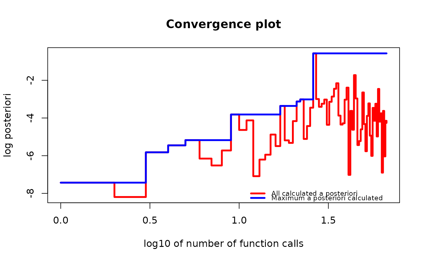
plot(g_map, type = "both", logarithmic_x = TRUE)