gips - Gaussian model Invariant by Permutation Symmetry
gips is an R package that looks for permutation symmetries in the multivariate Gaussian sample. Such symmetries reduce the free parameters in the unknown covariance matrix. This is especially useful when the number of variables is substantially larger than the number of observations.
gips will help you with two things:
- Finding hidden symmetries between the variables.
gipscan be used as an exploratory tool for searching the space of permutation symmetries of the Gaussian vector. Useful in the Exploratory Data Analysis (EDA). - Covariance estimation. The Maximum Likelihood Estimator (MLE) for the covariance matrix is known to exist if and only if the number of variables is less or equal to the number of observations. Additional knowledge of symmetries significantly weakens this requirement. Moreover, the reduction of model dimension brings the advantage in terms of precision of covariance estimation.
Installation
From CRAN:
# Install the released version from CRAN:
install.packages("gips")
From GitHub:
# Install the development version from GitHub:
# install.packages("remotes")
remotes::install_github("PrzeChoj/gips")
Examples
Example 1 - EDA
Assume we have the data, and we want to understand its structure:
library(gips)

Z <- HSAUR2::aspirin

# Renumber the columns for better readability:
Z[, c(2, 3)] <- Z[, c(3, 2)]
Assume the data Z is normally distributed.
dim(Z)
#> [1] 7 4
number_of_observations <- nrow(Z) # 7
p <- ncol(Z) # 4

S <- cov(Z)
round(S, -3)
#>         [,1]    [,2]    [,3]    [,4]
#> [1,]  381000  347000 1834000 1814000
#> [2,]  347000  317000 1675000 1659000
#> [3,] 1834000 1675000 8958000 8844000
#> [4,] 1814000 1659000 8844000 8755000

g <- gips(S, number_of_observations)
plot_cosmetic_modifications(plot(g, type = "heatmap"))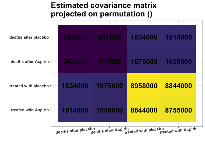
Remember, we analyze the covariance matrix. We can see some nearly identical colors in the estimated covariance matrix. E.g., variances of columns 1 and 2 are very similar (S[1,1] S[2,2]), and variances of columns 3 and 4 are very similar (S[3,3] S[4,4]). What is more, Covariances are also similar (S[1,3] S[1,4] S[2,3] S[2,4]). Are those approximate equalities coincidental? Or do they reflect some underlying data properties? It is hard to decide purely by looking at the matrix.
find_MAP() will use the Bayesian model to quantify if the approximate equalities are coincidental. Let’s see if it will find this relationship:
g_MAP <- find_MAP(g, optimizer = "brute_force")
#> ================================================================================

g_MAP
#> The permutation (1,2)(3,4):
#>  - was found after 17 posteriori calculations;
#>  - is 3.374 times more likely than the () permutation.
The find_MAP found the relationship (1,2)(3,4). The variances [1,1] and [2,2] as well as [3,3] and [4,4] are so close to each other that it is reasonable to consider them equal. Similarly, the covariances [1,3] and [2,4]; just as covariances [2,3] and [1,4], also will be considered equal:
S_projected <- project_matrix(S, g_MAP)
round(S_projected)
#>         [,1]    [,2]    [,3]    [,4]
#> [1,]  349160  347320 1746602 1744545
#> [2,]  347320  349160 1744545 1746602
#> [3,] 1746602 1744545 8856368 8844312
#> [4,] 1744545 1746602 8844312 8856368

plot_cosmetic_modifications(plot(g_MAP, type = "heatmap"))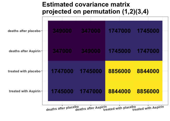
This S_projected matrix can now be interpreted as a more stable covariance matrix estimator.
We can also interpret the output as suggesting that there is no change in covariance for treatment with Aspirin.
Example 2 - modeling
First, construct data for the example:
# Prepare model, multivariate normal distribution
p <- 6
n <- 4
mu <- numeric(p)
sigma_matrix <- matrix(
  data = c(
    1.1, 0.8, 0.6, 0.4, 0.6, 0.8,
    0.8, 1.1, 0.8, 0.6, 0.4, 0.6,
    0.6, 0.8, 1.1, 0.8, 0.6, 0.4,
    0.4, 0.6, 0.8, 1.1, 0.8, 0.6,
    0.6, 0.4, 0.6, 0.8, 1.1, 0.8,
    0.8, 0.6, 0.4, 0.6, 0.8, 1.1
  ),
  nrow = p, byrow = TRUE
) # sigma_matrix is a matrix invariant under permutation (1,2,3,4,5,6)


# Generate example data from a model:
Z <- withr::with_seed(2022,
  code = MASS::mvrnorm(n, mu = mu, Sigma = sigma_matrix)
)
# End of prepare model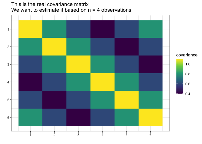
Suppose we do not know the actual covariance matrix and we want to estimate it. We cannot use the standard MLE because it does not exists (, ).
We will assume it was generated from the normal distribution with the mean .
library(gips)
dim(Z)
#> [1] 4 6
number_of_observations <- nrow(Z) # 4
p <- ncol(Z) # 6

# Calculate the covariance matrix from the data:
S <- (t(Z) %*% Z) / number_of_observations
Make the gips object out of data:
g <- gips(S, number_of_observations, was_mean_estimated = FALSE)We can see the standard estimator of the covariance matrix: It is not MLE (again, because MLE does not exist for ):
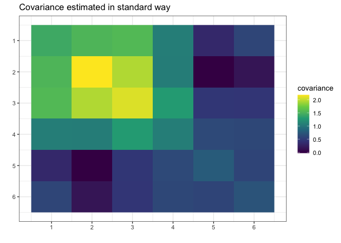
Let’s find the Maximum A Posteriori Estimator for the permutation. Space is small (), so it is reasonable to browse the whole of it:
g_map <- find_MAP(g, optimizer = "brute_force")
#> ================================================================================

g_map
#> The permutation (1,2,3,4,5,6):
#>  - was found after 362 posteriori calculations;
#>  - is 118.863 times more likely than the () permutation.
We see that the found permutation is 118.86 times more likely than making no additional assumption. That means the additional assumptions are justified.
What is more, we see the number of observations (4) is bigger than or equal to , so we can estimate the covariance matrix with the Maximum Likelihood estimator:
S_projected <- project_matrix(S, g_map)
S_projected
#>           [,1]      [,2]      [,3]      [,4]      [,5]      [,6]
#> [1,] 1.3747718 1.0985729 0.6960213 0.4960295 0.6960213 1.0985729
#> [2,] 1.0985729 1.3747718 1.0985729 0.6960213 0.4960295 0.6960213
#> [3,] 0.6960213 1.0985729 1.3747718 1.0985729 0.6960213 0.4960295
#> [4,] 0.4960295 0.6960213 1.0985729 1.3747718 1.0985729 0.6960213
#> [5,] 0.6960213 0.4960295 0.6960213 1.0985729 1.3747718 1.0985729
#> [6,] 1.0985729 0.6960213 0.4960295 0.6960213 1.0985729 1.3747718

# Plot the found matrix:
plot(g_map, type = "heatmap") + ggplot2::ggtitle("Covariance estimated with `gips`")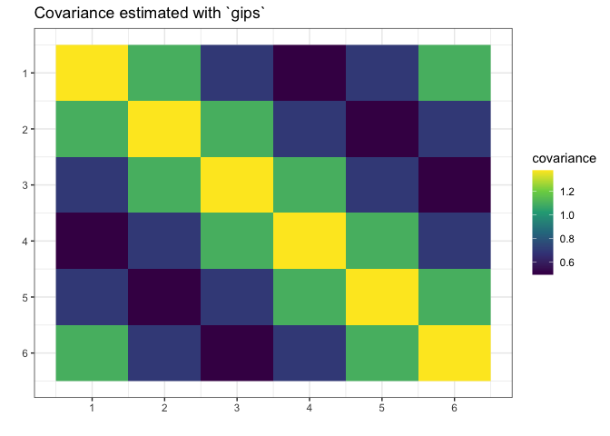
We see gips found the data’s structure, and we could estimate the covariance matrix with huge accuracy only with a small amount of data and additional reasonable assumptions.
Note that the rank of the S matrix was 4, while the rank of the S_projected matrix was 6 (full rank).
Further reading
For more examples and introduction, see vignette("gips", package="gips") or its pkgdown page.
For an in-depth analysis of the package performance, capabilities, and comparison with similar packages, see the article “Learning permutation symmetries with gips in R” by gips developers Adam Chojecki, Paweł Morgen, and Bartosz Kołodziejek, Journal of Statistical Software.
Acknowledgment
Project was funded by Warsaw University of Technology within the Excellence Initiative: Research University (IDUB) programme.
The development was carried out with the support of the Laboratory of Bioinformatics and Computational Genomics and the High Performance Computing Center of the Faculty of Mathematics and Information Science Warsaw University of Technology.