Plot optimized matrix or optimization gips object

Plot the heatmap of the MAP covariance matrix estimator or the convergence of the optimization method. The plot depends on the type argument.

Usage

# S3 method for class 'gips'
plot(
  x,
  type = NA,
  logarithmic_y = TRUE,
  logarithmic_x = FALSE,
  color = NULL,
  title_text = "Convergence plot",
  xlabel = NULL,
  ylabel = NULL,
  show_legend = TRUE,
  ylim = NULL,
  xlim = NULL,
  ...
)

Arguments

x

Object of a gips class.

type

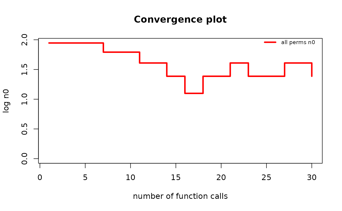
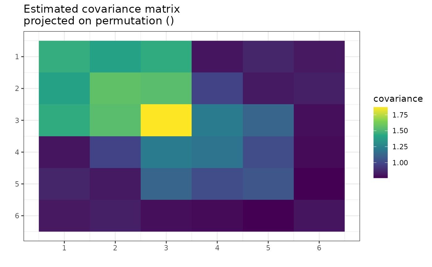
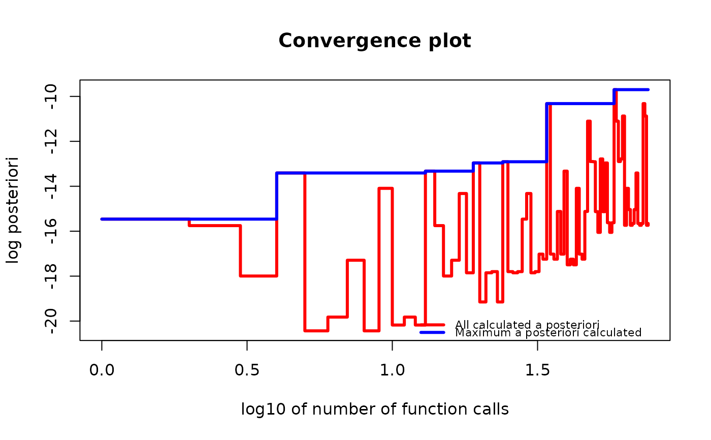
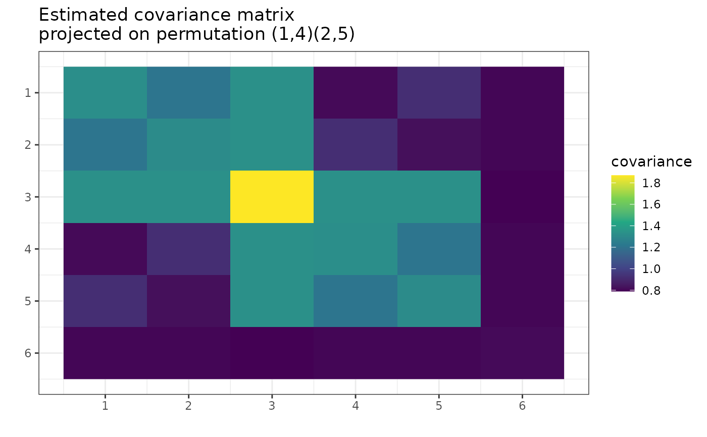
A character vector of length 1. One of c("heatmap", "MLE", "best", "all", "both", "n0", "block_heatmap"):

"heatmap", "MLE" - Plots a heatmap of the Maximum Likelihood Estimator of the covariance matrix given the permutation. That is, the S matrix inside the gips object projected on the permutation in the gips object.
"best" - Shows the maximum A Posteriori value found over time.
"all" - Shows the A Posteriori values for all visited states.
"both" - Shows both trajectories from "all" and "best".
"n0" - Plots the n0 values observed during optimization (only for "MH" optimization).
"block_heatmap" - Plots a heatmap of diagonally block representation of S. Non-block entries (equal to 0) are white for better clarity. For more information, see Block Decomposition - [1], Theorem 1 section in vignette("Theory", package = "gips") or in its pkgdown page.

The default value is NA, which will be changed to "heatmap" for non-optimized gips objects and to "both" for optimized ones. Using the default produces a warning.

Arguments logarithmic_y, logarithmic_x, color, title_text, xlabel, ylabel, show_legend, ylim, and xlim are only used for type %in% c("all", "best", "both", "n0") and ignored for heatmap types.

logarithmic_y, logarithmic_x

A boolean. Sets the axis of the plot in logarithmic scale. Only used for type %in% c("all", "best", "both", "n0").

color

Vector of colors to be used to plot lines. Only used for type %in% c("all", "best", "both", "n0").

title_text

Text to be in the title of the plot. Only used for type %in% c("all", "best", "both", "n0").

xlabel

Text to be on the bottom of the plot. Only used for type %in% c("all", "best", "both", "n0").

ylabel

Text to be on the left of the plot. Only used for type %in% c("all", "best", "both", "n0").

show_legend

A boolean. Whether or not to show a legend. Only used for type %in% c("all", "best", "both", "n0").

ylim

Limits of the y axis. When NULL, uses the data range. Only used for type %in% c("all", "best", "both", "n0").

xlim

Limits of the x axis. When NULL, uses the data range. Only used for type %in% c("all", "best", "both", "n0").

...

Ignored.

Value

An object of class ggplot.

Examples

require("MASS") # for mvrnorm()

perm_size <- 6
mu <- runif(6, -10, 10) # Assume we don't know the mean
sigma_matrix <- matrix(
  data = c(
    1.0, 0.8, 0.6, 0.4, 0.6, 0.8,
    0.8, 1.0, 0.8, 0.6, 0.4, 0.6,
    0.6, 0.8, 1.0, 0.8, 0.6, 0.4,
    0.4, 0.6, 0.8, 1.0, 0.8, 0.6,
    0.6, 0.4, 0.6, 0.8, 1.0, 0.8,
    0.8, 0.6, 0.4, 0.6, 0.8, 1.0
  ),
  nrow = perm_size, byrow = TRUE
) # sigma_matrix is a matrix invariant under permutation (1,2,3,4,5,6)
number_of_observations <- 13
Z <- MASS::mvrnorm(number_of_observations, mu = mu, Sigma = sigma_matrix)
S <- cov(Z) # Assume we have to estimate the mean

g <- gips(S, number_of_observations)
plot(g, type = "MLE")


g_map <- find_MAP(g, max_iter = 30, show_progress_bar = FALSE, optimizer = "hill_climbing")
plot(g_map, type = "both", logarithmic_x = TRUE)


plot(g_map, type = "MLE")

# Now, the output is (most likely) different because the permutation
  # `g_map[[1]]` is (most likely) not an identity permutation.

g_map_MH <- find_MAP(g, max_iter = 30, show_progress_bar = FALSE, optimizer = "MH")
plot(g_map_MH, type = "n0", logarithmic_y = FALSE)

Plot optimized matrix or optimization `gips` object

Usage

Arguments

Value

See also

Examples